Tutorial: Getting Started with Machine Learning in Python

Machine learning is definitely on the rise nowadays. The ability of computers to learn from examples instead of operating strictly according to previously written rules is an exciting way of solving problems.

Python is the most popular language for machine learning and data science. In this article we will show the basic tool chain for implementing machine learning in Python.

We will explain:

• how to load a data set
• how to run a machine learning algorithm on the data
• how to assess the performance of the algorithm

...all in just few lines of Python code!

But first, a disclaimer. We want to show you in practice how to take your first steps with machine learning without getting drowned in theory. So we will only give you the ‘need-to-know’ of what machine learning is.

We will not explain how the algorithm works. We will not show how to choose the right algorithm for your problem. Nor will we present how to optimize the parameters of the algorithm.

We will concentrate on the basics and we are going to go over the process of machine learning on a concrete example from A (getting data) to Z (evaluating the performance [accuracy] of the created model).

We assume that the reader has a rough knowledge about what machine learning is about and that he knows Python already.

We hope that by the end of this article you will be able to see why Python is the number one choice for this domain.

The goal of this article is to show machine learning on an approachable example. An important issue you need to solve at the beginning is acquiring a dataset.

Luckily, there are large datasets publicly available for use and they are extremely useful for starting your adventure in machine learning.

For this article we chose a problem that can be researched using a public dataset (more information about acquiring it later).

The example problem we would like to tackle with machine learning is the following:

Based on a person's attributes (like age, working hours, industry sector, etc.), predict whether the person has a high salary or not (whether they earn more or less than 50,000 USD per year).

This problem is a classification problem. We want to categorize the population into two classes: high-income and low-income. Since there are only two classes and each person belongs to exactly one class we call it a binary classification problem.

In other words, for each person we are trying to determine whether they belong to the low-income class or not.

The process of machine learning can be split into the following steps:

Machine learning overview

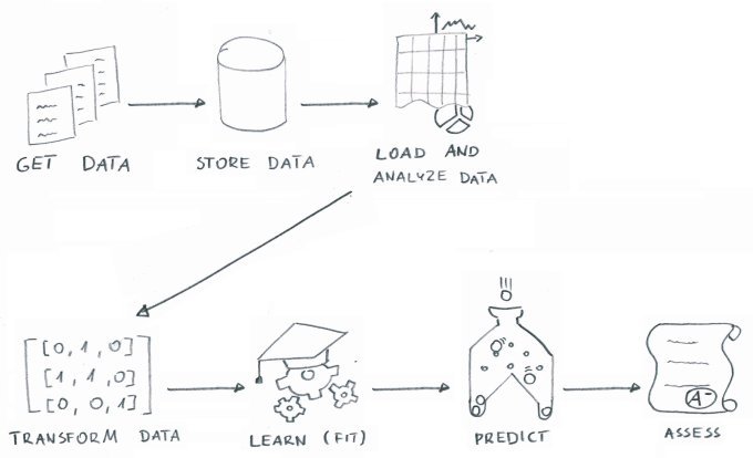
a) Get data

Acquire a big enough dataset (including labels or answers to your problem).

b) Store data

Store the acquired data in a single location for easy retrieval.

c) Load and analyze data

Load your dataset from storage and do basic data analysis and visualization.

d) Transform data

Machine learning requires purely numeric input, so you need to transform the input data.

e) Learn (fit)

Run the labeled data through a machine learning algorithm yielding a model.

f) Predict

Use the model to predict labels for data that the model did not see previously.

g) Assess

Verify the accuracy of predictions made by the model.

In order to start the machine learning process you need to possess a set of data to be used for training the algorithm.

It's very important to ensure that the source of data is credible, otherwise you would receive incorrect results, even if the algorithm itself is working correctly (following the garbage in, garbage out principle).

The second important thing is the size of the dataset. There is no straightforward answer for how large it should be. The answer may depend on many factors, for example:

• the type of problem you're looking to solve,
• the number of features in the data,
• the type of algorithm used.

Fortunately, it shouldn't be difficult to find a ready-made dataset for your example project.

For starters you may use one of built-in datasets provided by scikit-learn package.

A popular choice is the Iris flower dataset that consists of data on petal and sepal length for 3 different types of irises (Setosa, Versicolour, and Virginica), stored in a 150×4 numpy.ndarray:

>>> from sklearn import datasets
>>> iris = datasets.load_iris()
>>> print(iris.DESCR)
Iris Plants Database
====================

Notes
-----
Data Set Characteristics:
    :Number of Instances: 150 (50 in each of three classes)
    :Number of Attributes: 4 numeric, predictive attributes and the class
    :Attribute Information:
        - sepal length in cm
        - sepal width in cm
        - petal length in cm
        - petal width in cm
        - class:
                - Iris-Setosa
                - Iris-Versicolour
                - Iris-Virginica
...

>>> iris.data[:5]
array([[ 5.1,  3.5,  1.4,  0.2],
       [ 4.9,  3. ,  1.4,  0.2],
       [ 4.7,  3.2,  1.3,  0.2],
       [ 4.6,  3.1,  1.5,  0.2],
       [ 5. ,  3.6,  1.4,  0.2]])

Another good source of interesting publicly available datasets is the UC Irvine Machine Learning Repository which contains a vast collection of datasets used throughout the machine learning community.

For the purposes of this article we chose the Adult Data Set that contains 48,842 records extracted from the US 1994 Census database. Each record contains 14 attributes:

• age - integer,
• workclass - categorical values ('Private', 'Self-emp-not-inc', 'Self-emp-inc', 'Federal-gov', ...),
• fnlwgt - integer,
• education - categorical ('Bachelors', 'Some-college', '11th', 'HS-grad', ...),
• education-num - integer,
• marital-status - categorical ('Married-civ-spouse', 'Divorced', 'Never-married', 'Separated', ...),
• occupation - categorical ('Tech-support', 'Craft-repair', 'Other-service', 'Sales', ...),
• relationship - categorical ('Wife', 'Own-child', 'Husband', 'Not-in-family', ...),
• race - categorical ('White', 'Asian-Pac-Islander', 'Amer-Indian-Eskimo', 'Other', ...),
• sex - categorical ('Female', 'Male'),
• capital-gain - integer,
• capital-loss - integer,
• hours-per-week - integer,
• native-country - categorical ('United-States', 'Cambodia', 'England', 'Puerto-Rico', ...).

For each record we also get the classification label (<=50k or >50k - information about the yearly salary bracket).

Based on this dataset we're going to train a classification algorithm to be able to predict whether a person with a given set of attributes earns more or less than 50 thousand dollars per year.

After training your model, you will surely want to know if it is good enough at solving the problem in the real world.

To correctly measure the accuracy of your model, you need to validate it against a new set of data - different than the set your were training it with.

Thus, before using the collected dataset for training your algorithm, you should split it into a subset which will be used for the training process (training set) and a subset that will be used for validating the accuracy of the algorithm (test set).

In practice, you should devote 20%-30% of your collected dataset for validation purposes (test set).

Suppose you have a matrix of input data X and a vector of corresponding expected results y. You can use a simple utility function: sklearn.model_selection.train_test_split to split it into a train and test subsets with the given proportion:

from sklearn.model_selection import train_test_split

X_train, X_test, y_train, y_test = train_test_split(X, y, test_size=0.25)

For our example problem we don't have to split the dataset on our own. The Adult Data Set collection we chose already consists of two separate files:

• training set – adult.data (32,561 records)
• test set – adult.test (16,281 records)

Disclaimer: we omit the description of loading data from text files downloaded from the UC Irvine Machine Learning Repository into a SQLite database because that is outside the scope of this article. You can still read our solution yourself in the Complete listing section.

Once you have your data stored in a single location you should load them into a tool that will allow you to analyze it easily, slice'n'dice them and later on use them with your machine learning algorithm.

The Python pandas package is a great tool for that.

Out of the box it allows you to read your data from a variety of formats:

• flat files such as CSV, JSON, HTML,
• binary formats including Excel and pickle,
• relational databases,
• cloud (Google Big Query),
• and others.

Below we present an example of reading data from an SQL database through SQLAlchemy.

import os.path
import pandas
from sqlalchemy import create_engine

def read_data_frame():
    DB_FILE_PATH = os.path.join(os.path.dirname(__file__), 'data.sqlite')
    TABLE_NAME = 'adult'
    engine = create_engine(f'sqlite:///{DB_FILE_PATH}')
    with engine.connect() as conn:
        with conn.begin():
            return pandas.read_sql_table(TABLE_NAME, conn, index_col='id')

The data is read as a pandas DataFrame object. The object contains information about properties (columns) in the data:

>>> data_frame.columns
Index(['age', 'workclass', 'fnlwgt', 'education', 'education_num',
       'marital_status', 'occupation', 'relationship', 'race', 'sex',
       'capital_gain', 'capital_loss', 'hours_per_week', 'native_country',
       'classification'],
      dtype='object')

You can view a data record:

>>> data_frame.iloc[0]
age                          39
workclass             State-gov
fnlwgt                    77516
education             Bachelors
education_num                13
marital_status    Never-married
occupation         Adm-clerical
relationship      Not-in-family
race                      White
sex                        Male
capital_gain               2174
capital_loss                  0
hours_per_week               40
native_country    United-States
classification            <=50K
Name: 1, dtype: object

You can view the data column by column:

>>> data_frame.workclass
id
1               State-gov
2        Self-emp-not-inc
3                 Private
4                 Private
5                 Private
6                 Private
7                 Private
8        Self-emp-not-inc
9                 Private
10                Private
               ...
32552             Private
32553             Private
32554             Private
32555             Private
32556             Private
32557             Private
32558             Private
32559             Private
32560             Private
32561        Self-emp-inc
Name: workclass, Length: 32561, dtype: object

You can quickly get a summary of value counts for a specific column:

>>> data_frame.workclass.value_counts()
Private             22696
Self-emp-not-inc     2541
Local-gov            2093
?                    1836
State-gov            1298
Self-emp-inc         1116
Federal-gov           960
Without-pay            14
Never-worked            7
Name: workclass, dtype: int64

The pandas library enables you to group, filter, transform your data and much, much more.

Before you start modeling the data it may be very beneficial to visualize it. It will let you better understand the nature of the data you're going to work with. You might find relationships and patterns between input values which will help you get better results.

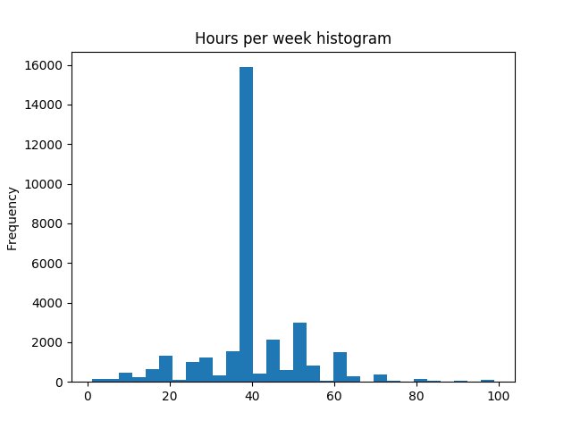
Data visualization may also help you to pre-validate the input data. For example, you would expect that most people work 40 hours a week. In order to examine if your assumption is correct you could draw a histogram chart. You can do it quickly using the matplotlib plotting library integrated with your pandas DataFrame:

import matplotlib.pyplot as plt

data_frame.hours_per_week.plot.hist(bins=30)
plt.show()

It should display the following chart:

Hours per week histogram

A quick look at the generated chart confirms that your assumption was correct.

Suppose you would like to see how age and the number of hours worked per week correlate with earnings. For that your can make matplotlib draw a scatter plot of your data:

import numpy as np

colors = np.where(data_frame.classification == '>50K', 'r', 'k')
plot = data_frame.plot.scatter(x='age', y='hours_per_week', s=10, c=colors)
plot.figure.show()

As a result you receive a chart showing correlation between values from two columns of your collection (age and number of hours worked per week) where the red dots represents people whose yearly earnings are higher and black dots lower than $50,000:

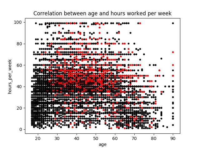
Scatter plot example

You can see that the density of red dots is higher in the area represented by samples of people between 30 and 60 years where the hours worked per week is above 40.

As you can see matplotlib is a powerful and easy to use library which can be very useful for visualizing the processed data. Moreover, it's nicely wrapped by Series and DataFrame objects which are used for representing datasets in pandas library, which makes plotting different kinds of charts even more handy.

a) Mapper

The machine learning algorithm expects only numerical values as input. To be exact, it expects a numpy low-level matrix of numerical data.

The data we loaded earlier is stored in a pandas DataFrame. To transform the DataFrame into the numpy array we need, we can use DataFrameMapper from sklearn-pandas - a library that bridges the gap between pandas and sklearn.

The mapper allows us to select which data attributes (columns) we want to use for machine learning and what transformations should be performed for each attribute. Each column can have one or multiple transformations applied in turn:

import sklearn.preprocessing
from sklearn_pandas import DataFrameMapper

mapper = DataFrameMapper([
    (['age'], sklearn.preprocessing.StandardScaler()), # single transformation
    ('sex', sklearn.preprocessing.LabelBinarizer()), # single transformation
    ('native_country', [ # multiple transformations
        sklearn.preprocessing.FunctionTransformer(
            native_country_generalize, validate=False
        ),
        sklearn.preprocessing.LabelBinarizer()
    ]),
    ...
])

If the column does not need any transformations use None in the configuration for that attribute. Attributes not mentioned in the mapper configuration will not be used in the mapper's output.

In our data we have some numerical attributes (for example age) as well as some string enumerations (for example sex, marital_status).

b) Scaling numerical values

It is a good practice to scale all numerical values to a standard range to avoid problems when one attribute (for example capital_gain) would outweigh another's importance (for example age) due to its values' higher order of magnitude. We can use sklearn.preprocessing.StandardScaler to scale the values for us.

c) Transforming enumerations

Enumerations are a more complex case. If the enumeration only has 2 possible values:

we can convert the column to a boolean flag column:

If the enumeration has more values, for example:

then we can transform it into a series of boolean flag columns, one for each possible enumeration value:

sklearn.preprocessing.LabelBinarizer can handle both of the scenarios listed above.

d) Complex transformations

Sometimes we want to run a more advanced transformation on data including applying some business logic. In our data the attribute native_country has 42 possible values, though 90% of the records contain the value United-States.

To avoid creating 42 new columns, we would like to reduce the column to contain a smaller set of values: United-States and Other for the 10% remaining records. We can use sklearn.preprocessing.FunctionTransformer to achieve this:

import numpy
import functools

def numpy_map(callback):
    @functools.wraps(callback)
    def numpy_map_wrapper(X):
        return numpy.array([callback(x) for x in X])
    return numpy_map_wrapper

@numpy_map
def native_country_generalize(x):
    return 'US' if x == 'United-States' else 'Other'

mapper = DataFrameMapper([
    ...
    ('native_country', [
        sklearn.preprocessing.FunctionTransformer(
            native_country_generalize, validate=False
        ),
        sklearn.preprocessing.LabelBinarizer()
    ])
])

Notice how we are still running the output of the FunctionTransformer through LabelBinarizer to convert new enumerations to boolean flags.

e) Features

The DataFrameMapper converts our pandas DataFrame into a numpy matrix of features. A feature is a single input to our machine learning algorithm.

As you could see, one column of our original data can correspond to more than one feature (in the case of enumerations).

If you would like to preview the output that the mapper is producing, you can run it on the training data inputs:

>>> data = mapper.fit_transform(train_X)
>>> data
array([[ 0.03067056,  1.        ,  0.        , ..., -0.21665953,
        -0.03542945,  1.        ],
       [ 0.83710898,  0.        ,  0.        , ..., -0.21665953,
        -2.22215312,  1.        ],
       [-0.04264203,  0.        ,  0.        , ..., -0.21665953,
        -0.03542945,  1.        ],
       ...,
       [ 1.42360965,  0.        ,  0.        , ..., -0.21665953,
        -0.03542945,  1.        ],
       [-1.21564337,  0.        ,  0.        , ..., -0.21665953,
        -1.65522476,  1.        ],
       [ 0.98373415,  0.        ,  0.        , ..., -0.21665953,
        -0.03542945,  1.        ]])
>>> data.dtype
dtype('float64')

You can see that the mapper produced a two-dimensional numpy matrix of floating point values. This is the format of input that the machine learning algorithm expects.

However, this data is just a collection of numbers. It does not store information about column names or enumeration values. In other words, the data in this format is hardly human readable. It would be difficult to analyze the data in this state. That's why we’d rather use pandas to load and play with the data, and execute this transformation only just before running the algorithm.

Having the input data pre-processed, you're ready to provide it to the chosen algorithm in order to train the model.

In our presented example we decided to use the Multi-layer Perceptron (MLP) algorithm, which is an example of a supervised learning neural network classification algorithm. We won't be focusing on the details of the algorithm selection process in this article, however you should be aware that it depends on the type of problem you need to solve and the type and volume of data you possess.

A supervised learning algorithm is an approach that requires the training data to contain both the input object (a vector of features) and the expected output value for this object. Thus, we need to split our train_data_frame into:

• train_X – a DataFrame object containing input records with the classification column omitted
• train_y – a Series object containing only the classification column (mapped into boolean values)

classification_map = {
    '<=50K': True,
    '>50K': False
}

train_X = train_data_frame[train_data_frame.columns.drop('classification')]
train_y = train_data_frame['classification'].map(classification_map)

The classifier object (sklearn.neural_network.MLPClassifier) must be initialized with a number of parameters, such as the number of hidden layers of the neural network or their sizes (i.e. the number of neurons in each layer). For the sake of conciseness, we don't show how to determine the best values for those parameters. Take our word for it that the best accuracy for this problem can be achieved by a neural network consisting of 1 hidden layer containing 20 neurons.

from sklearn.neural_network import MLPClassifier

NUMBER_OF_LAYERS = 1
NEURONS_PER_LAYER = 20

classifier = MLPClassifier(
    hidden_layer_sizes=(NEURONS_PER_LAYER, ) * NUMBER_OF_LAYERS,
    alpha=0.01,
    random_state=1
)

Finally, we apply the training data to the classifier algorithm. Before we do that, we use our previously constructed mapper to transform the input the data into the numeric form to be understood by the classifier object.

from sklearn.pipeline import Pipeline

pipeline = Pipeline([
    ('mapper', mapper),
    ('classifier', classifier)
])

model = pipeline.fit(X=train_X, y=train_y)

According to the scikit-learn documentation - all supervised estimators implement a fit(X, y) method to fit (train) the model and a predict(X) method that, given unlabeled observations X, returns the predicted labels y.

The classification model produced as a result of the training process can be now used to predict the classification on the test set DataFrame or possibly totally new data out in the wild.

test_X = test_data_frame[test_data_frame.columns.drop('classification')]

predictions = model.predict(X=test_X)

The last step you should take is model evaluation. This will tell you how accurate the predictions made by the trained model are.

As you might notice, the evaluation process is executed on the previously extracted test set (test_X, test_y) which was not seen by the model earlier, during the training process.

You should never evaluate the model on the train set, because the results obtained would not translate into real world applications (in that way you wouldn't be able to verify if your model is able to make generalizations).

There are a couple of metrics that let you evaluate the accuracy of your model. The most basic one is sklearn.metrics.accuracy_score which represents a ratio of all correctly predicted values to all processed samples.

from sklearn import metrics

test_y = test_data_frame['classification'].map(classification_map)

accuracy_score = metrics.accuracy_score(test_y, predictions)

In our example, the accuracy_score returns the value of 0.856212763344 which can be interpreted as "~85% of predictions are correct".

We showed you how to run your first machine learning algorithm on an example dataset. By evaluating the created model we proved that machine learning works (85% accuracy is not a bad result).

What you should have noticed throughout the article is that we didn't write that much code. Certainly we didn't have to write the machine learning algorithm itself.

For each task along the way we had a ready-to-use, battle-tested Python library to do the heavy lifting for us:

• pandas for loading and playing around with data,
• matplotlib for visualizing the data,
• sklearn-pandas for transforming our inputs into a numerical matrix,
• sklearn for the actual machine learning and assessment.

What we had to write was just the glue-code that tied everything together.

And that's why Python is the number one language for doing machine learning - all the tools are there, the usage is simple, the documentation extensive and the community vibrant. You can have a machine learning solution running in no time!

Below you can find the complete machine learning script used for this article.

import csv
import functools
import os.path

import numpy
from sqlalchemy import create_engine
import pandas
from sklearn_pandas import DataFrameMapper
import sklearn.preprocessing
from sklearn.pipeline import Pipeline
from sklearn.neural_network import MLPClassifier
from sklearn import metrics


DIR = '/home/user/workspace/machine-learning'

TRAIN_DATA_FILE_PATH = os.path.join(DIR, 'data', 'adult.data')
TEST_DATA_FILE_PATH = os.path.join(DIR, 'data', 'adult.test')

TRAIN_DB_FILE_PATH = os.path.join(DIR, 'db', 'data.sqlite')
TEST_DB_FILE_PATH = os.path.join(DIR, 'db', 'test.sqlite')

train_engine = create_engine(f'sqlite:///{TRAIN_DB_FILE_PATH}')
test_engine = create_engine(f'sqlite:///{TEST_DB_FILE_PATH}')

INT = 'INTEGER'
STR = 'VARCHAR'

FIELDS = (
    ('age', INT),
    ('workclass', STR),
    ('fnlwgt', INT),
    ('education', STR),
    ('education_num', INT),
    ('marital_status', STR),
    ('occupation', STR),
    ('relationship', STR),
    ('race', STR),
    ('sex', STR),
    ('capital_gain', INT),
    ('capital_loss', INT),
    ('hours_per_week', INT),
    ('native_country', STR),
    ('classification', STR)
)


def create_schema(connection):
    fields_sql = ', '.join(
        f'{field_name} {field_type}' for (field_name, field_type) in FIELDS
    )
    connection.execute(
        f'CREATE TABLE adult (id INTEGER PRIMARY KEY, {fields_sql})'
    )


def read_data(data_file_path):
    with open(data_file_path, newline='') as csvfile:
        reader = csv.reader(csvfile, delimiter=',', skipinitialspace=True)
        for row in reader:
            if len(row) != 15:
                continue  # Skip empty rows, skip test file header
            classification = row[-1]
            if classification.endswith('.'):
                # Test file has dots ('.') at the end of lines, strip them out.
                row[-1] = classification[:-1]
            yield row


def insert_row(row, connection):
    fields = ', '.join(field_name for (field_name, _) in FIELDS)
    placeholders = ', '.join(['?'] * len(FIELDS))
    connection.execute(
        f'INSERT INTO adult ({fields}) VALUES ({placeholders})', row
    )


def import_data(data, connection):
    create_schema(connection)
    with connection.begin():
        for row in data:
            insert_row(row, connection)


def gather_data():
    return read_data(TRAIN_DATA_FILE_PATH), read_data(TEST_DATA_FILE_PATH)


def store_data(train_data, test_data):
    with train_engine.connect() as conn:
        import_data(train_data, conn)
    with test_engine.connect() as conn:
        import_data(test_data, conn)


def load_data(train_engine, test_engine):
    with train_engine.connect() as conn:
        with conn.begin():
            train_data_frame = pandas.read_sql_table(
                'adult', conn, index_col='id'
            )

    with test_engine.connect() as conn:
        with conn.begin():
            test_data_frame = pandas.read_sql_table(
                'adult', conn, index_col='id'
            )

    return train_data_frame, test_data_frame


def get_mapper():
    def numpy_map(callback):
        @functools.wraps(callback)
        def numpy_map_wrapper(X):
            return numpy.array([callback(x) for x in X])
        return numpy_map_wrapper

    @numpy_map
    def native_country_generalize(x):
        return 'US' if x == 'United-States' else 'Other'

    @numpy_map
    def workclass_generalize(x):
        if x in ['Self-emp-not-inc', 'Self-emp-inc']:
            return 'Self-emp'
        elif x in ['Local-gov', 'State-gov', 'Federal-gov']:
            return 'Gov'
        elif x in ['Without-pay', 'Never-worked', '?']:
            return 'None'
        else:
            return x

    @numpy_map
    def education_generalize(x):
        if x in ['Assoc-voc', 'Assoc-acdm']:
            return 'Assoc'
        elif x in [
            '11th', '10th', '7th-8th', '9th', '12th', '5th-6th',
            '1st-4th', 'Preschool'
        ]:
            return 'Low'
        else:
            return x

    return DataFrameMapper([
        (['age'], sklearn.preprocessing.StandardScaler()),
        ('workclass', [
            sklearn.preprocessing.FunctionTransformer(
                workclass_generalize, validate=False
            ),
            sklearn.preprocessing.LabelBinarizer()
        ]),
        # ('fnlwgt', None),
        ('education', [
            sklearn.preprocessing.FunctionTransformer(
                education_generalize, validate=False
            ),
            sklearn.preprocessing.LabelBinarizer()
        ]),
        (['education_num'], sklearn.preprocessing.StandardScaler()),
        ('marital_status', sklearn.preprocessing.LabelBinarizer()),
        ('occupation', sklearn.preprocessing.LabelBinarizer()),
        ('relationship', sklearn.preprocessing.LabelBinarizer()),
        ('race', sklearn.preprocessing.LabelBinarizer()),
        ('sex', sklearn.preprocessing.LabelBinarizer()),
        (['capital_gain'], sklearn.preprocessing.StandardScaler()),
        (['capital_loss'], sklearn.preprocessing.StandardScaler()),
        (['hours_per_week'], sklearn.preprocessing.StandardScaler()),
        ('native_country', [
            sklearn.preprocessing.FunctionTransformer(
                native_country_generalize, validate=False
            ),
            sklearn.preprocessing.LabelBinarizer()
        ]),
    ])


classification_map = {
    '<=50K': True,
    '>50K': False
}


def train(train_data_frame, mapper):
    train_X = train_data_frame[train_data_frame.columns.drop('classification')]
    train_y = train_data_frame['classification'].map(classification_map)

    NUMBER_OF_LAYERS = 1
    NEURONS_PER_LAYER = 20

    classifier = MLPClassifier(
        hidden_layer_sizes=(NEURONS_PER_LAYER, ) * NUMBER_OF_LAYERS,
        alpha=0.01,
        random_state=1
    )

    pipeline = Pipeline([
        ('mapper', mapper),
        ('classifier', classifier)
    ])

    model = pipeline.fit(X=train_X, y=train_y)
    return model


def predict(model, test_data_frame):
    test_X = test_data_frame[test_data_frame.columns.drop('classification')]

    predictions = model.predict(X=test_X)
    return predictions


def assess(test_data_frame, predictions):
    test_y = test_data_frame['classification'].map(classification_map)

    accuracy_score = metrics.accuracy_score(test_y, predictions)
    return accuracy_score


def main():
    train_data, test_data = gather_data()
    store_data(train_data, test_data)
    train_data_frame, test_data_frame = load_data(train_engine, test_engine)
    mapper = get_mapper()
    model = train(train_data_frame, mapper)
    predictions = predict(model, test_data_frame)
    score = assess(test_data_frame, predictions)
    print('Accuracy score', score)


if __name__ == '__main__':
    main()

cycler==0.10.0
matplotlib==2.1.1
numpy==1.13.3
pandas==0.21.1
pyparsing==2.2.0
python-dateutil==2.6.1
pytz==2017.3
scikit-learn==0.19.1
scipy==1.0.0
six==1.11.0
sklearn==0.0
sklearn-pandas==1.6.0
SQLAlchemy==1.1.15