


Project context: Measuring sponsor exposure in real sports footage
Our project started with a practical business goal: automatically measuring sponsor exposure in sports channel broadcasts. Traditionally, measuring brand visibility in sports is a manual, time-consuming process. Analysts sit through hours of video material to identify where sponsor logos appear and estimate how much exposure each brand received.
Before the ML pipeline can run, the video needs to be converted into image frames. This should be done with a consistent sampling strategy, for example taking frames at a fixed rate depending on how accurate the exposure timing needs to be. Higher sampling gives more precise exposure measurement but increases processing cost, while lower sampling is cheaper and usually sufficient for reporting trends across long broadcasts. Each extracted frame should keep its original timestamp, because the final sponsor report needs to translate model predictions back into real video time.
To automate this, the system had to process broadcast frames, locate sponsor logos, and classify each detected crop into a known brand. The output wasn't just a generic "a logo was found" event: it had to provide bounding box coordinates tied to clear brand identities for exposure-time reporting.
On paper, this sounds like a standard computer vision task: detect an object, crop it, classify it, and aggregate results. In practice, live broadcast video breaks almost every clean assumption that machine learning models rely on:
- Unconstrained placement: Logos appear on creased shirts, moving players, pitch-side LED boards, walls, banners, overlays, and background elements.
- Severe visual noise: Crops are frequently small, distorted by camera perspective, motion-blurred, or partially occluded by referees or players.
- Data inconsistencies: Some visible logos in the frames were completely unannotated in the ground truth. Furthermore, class distributions were heavily imbalanced – top sponsors had thousands of examples, while long-tail brands had fewer than ten.
The final production metric was a Sponsor Exposure Score. Instead of reporting only whether a logo was detected, the system aggregated detections over video time and calculated exposure per brand. Consecutive detections of the same sponsor were grouped into visibility intervals, then weighted by how prominent the logo was on screen and by model confidence. This gave the business team two practical outputs: total exposure time and a weighted exposure score that better reflected real sponsor visibility during the broadcast.
That reality dictated our core challenge: we needed a system architecture that could be continuously evaluated, updated, monitored, and scaled as sponsor sets and visual data changed over time.
Why a single end-to-end model fails in production
When designing a logo exposure system, the initial temptation is to train a single, monolithic model that localizes and classifies every target brand in one pass. For a fixed set of brands in a closed experiment, that approach looks cleaner.
However, in a live business domain, localization and classification evolve at completely different speeds:
- Localization is relatively stable: The features that make a bounding box "look like a logo" in a sports broadcast remain similar regardless of whether the sponsor is ORLEN, BMW, PGE, or an unknown local brand.
- Brand identity is highly dynamic: New sponsors get onboarded mid-season, existing brands refresh their visual identity, and human reviewers frequently need to correct mislabeled predictions.
If localization and identification live inside a single neural network, every single brand update or rebranding event forces a full model retraining cycle. That makes maintenance expensive and operationally fragile.
To solve this, we decoupled the task into two independent stages:
- Logo Detector: A 1-class detector responsible only for localization. It answers: "Does this region look like a logo?"
- Logo Classifier: A vector-based classifier responsible for brand identity. It answers: "Which known brand does this crop match, or is it UNCLASSIFIED?"
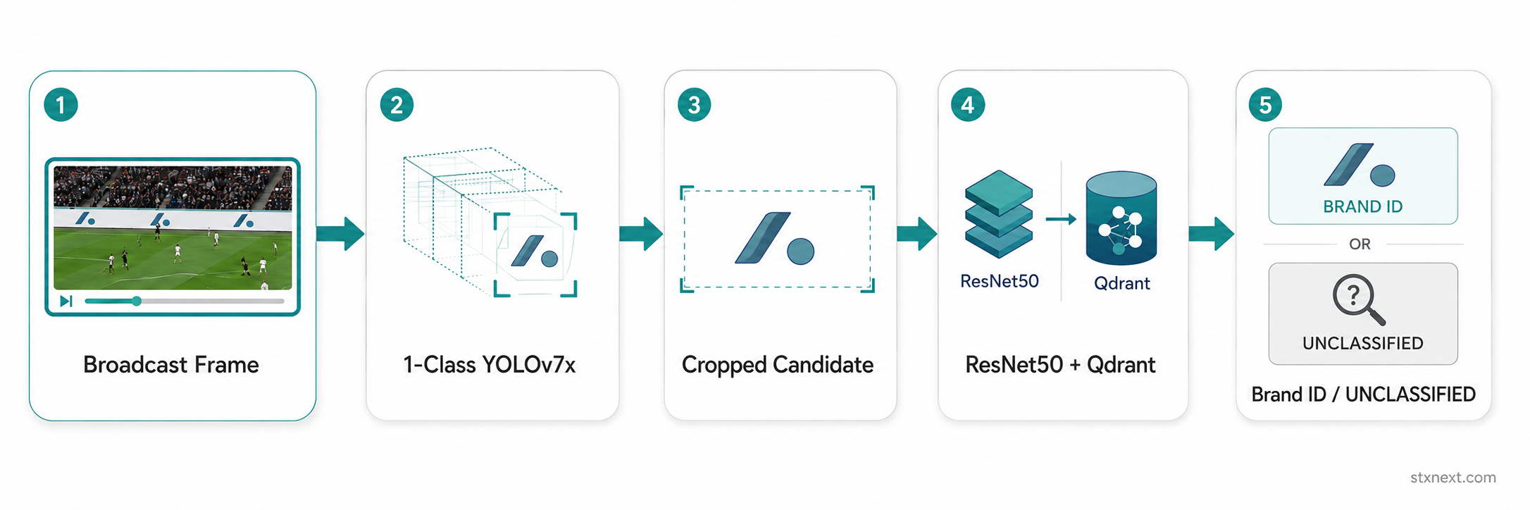
1. The detector: Finding logo locations & licensing traps
The detection stage used a one-class object detector trained on 6,924 sports video frames. The model was trained purely to output bounding boxes for any candidate logo region.
During training, we encountered a classic production issue: incomplete ground truth. Secondary logos (such as channel watermarks) appeared in frames but were omitted from the label files. When our detector correctly localized these logos, standard evaluation metrics penalized them as False Positives. This distinction is crucial for a production pipeline: a model can be visually correct while its offline evaluation metrics are artificially suppressed by incomplete annotations.
When selecting our detector backbone, experimental metrics collided directly with commercial constraints. We tested several YOLO-based configurations, including additional experiments around training setup and hyperparameter selection. The useful finding was that hyperparameter tuning did not improve detection performance: most modifications caused the metrics to drop, suggesting that the default YOLO training configuration was already a strong fit for this dataset:
Data augmentation was also used during detector training by pasting 3-10 small logos (50-100 px) into sparse image regions.
In the YOLOv7x experiments, controlled augmentation produced a small but consistent lift. The non-augmented YOLOv7x run reached mAP50 0.925, precision 0.894, recall 0.877, and F1 0.885. After adding controlled logo pasting, the augmented run reached mAP50 0.928, precision 0.901, recall 0.876, and F1 0.888.
The improvement was not dramatic, but it was useful. It showed that augmentation can help when synthetic logos preserve realistic placement, scale, and density. Later experiments also suggested that adding more synthetic data is not automatically better, so augmentation had to be treated as a controlled experiment rather than a guaranteed performance boost.
2. The classifier: Vector search over closed softmax
Once candidate logo regions were cropped, they were passed to the classification layer. Because these crops were noisy, varied in size, and frequently contained unknown logos, a traditional closed softmax classifier was insufficient.
Instead, we used a fine-tuned ResNet50 model to convert each logo crop into a 1024-dimensional visual embedding, storing these vectors in a Qdrant database. During inference, new crops were embedded and matched against known brand clusters.
We evaluated three retrieval strategies across a dataset scaled to 18,333 embedded examples:
- Nearest Neighbor (k=1): Highly vulnerable to visual noise, partial crops, and background clutter (achieved 61.98% baseline accuracy).
- Class Centroid: Smoothes out intra-class variance too aggressively. It failed because a brand logo printed on a wrinkled shirt looks visually distinct from the same logo on a flat LED wall.
- Neighborhood Consensus (k=4): Evaluates distance consensus among the 4 (tested also on 3 and 5) nearest vectors. This made classification less sensitive to outliers and mislabeled embeddings than single nearest-neighbor matching, making it the most resilient strategy in our experiments and improving accuracy to 90.28%.
We tested more classification variants than shown below, including different embedded datasets, thresholds, and retrieval strategies. The table summarizes only the key milestones that best explain how the classification stage improved from the initial baseline to the strongest tested setup.
3. Overcoming data imbalance & visual concept drift
Data imbalance was one of our primary performance bottlenecks in the classification stage. The training data included a large number of logo examples, but the distribution was highly uneven: some logo classes had only a few examples, often between 3 and 10 images, while others had several hundred or even thousands of crops.
This imbalance directly affected classification quality. Underrepresented classes initially plateaued at around 50–60% accuracy, compared to 80–98% for well-represented brands.
To mitigate this, we implemented three key adjustments:
- Circle loss: Employed during ResNet50 fine-tuning to optimize distance margins specifically for imbalanced vector spaces.
- Targeted augmentation: Applied rotation, blur, zoom, and color shifts strictly to classes with under 400 samples.
- Downsampling and oversampling: We also tested resampling strategies to reduce the impact of class imbalance between dominant sponsor classes and long-tail brands with only a few examples.
- K-means train/test splitting: K-means was used as a visual stratification strategy for the fixed classifier dataset prepared for the client. The goal was to split each brand into train and test sets while preserving similar proportions of visual variants inside the class. For example, if one logo appeared in different colors, layouts, or placements, clustering helped ensure that both train and test contained representative examples instead of accidentally testing only on a narrow visual subset.
Concept drift also manifested in concrete visual forms. Because brand identity evolved, monitoring drift via per-class recall became a mandatory operational requirement.
4. Production infrastructure, human feedback, and evaluation
Productionizing the system required around 14 weeks of ML engineering effort. The most challenging part was building a reliable logo-recognition workflow: training and evaluating the detector, fine-tuning the embedding model, designing the vector database layer, validating retrieval strategies, and creating feedback loops for correcting bad embeddings. REST APIs, batch processing, and dashboards were necessary production components which were built on top of it.
Three-tier evaluation pipeline
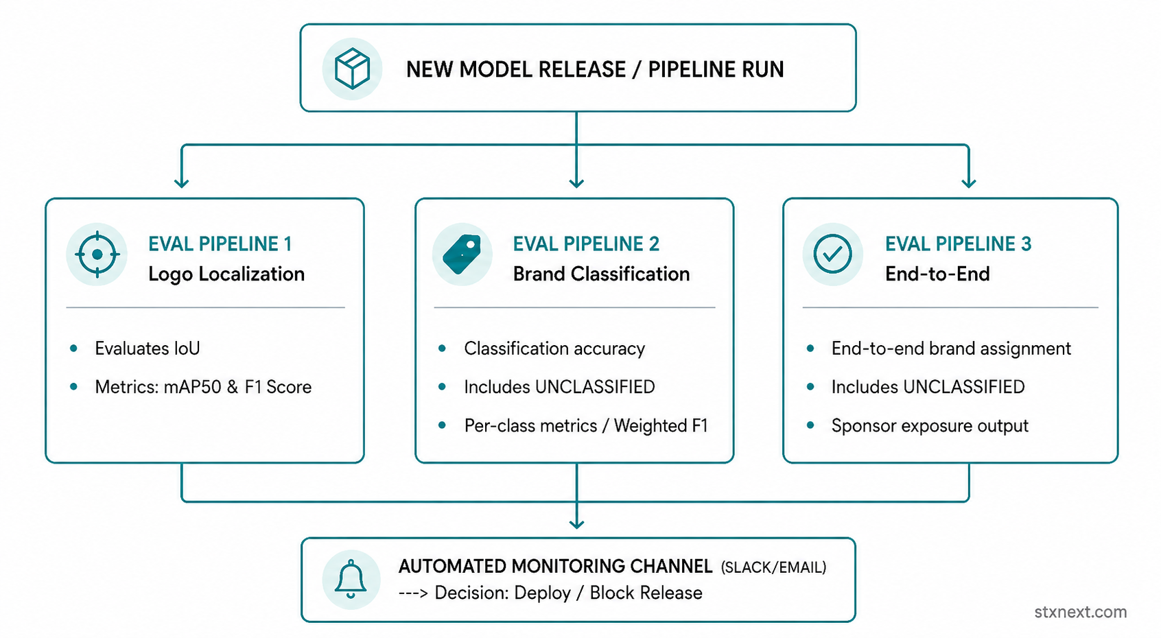
To deploy new model versions safely, we established three automated evaluation pipelines triggered on every release:
- Logo localization pipeline: Measures predicted-vs-ground-truth IoU and evaluates detection quality using mAP50, precision, recall, and F1 score.
- Logo classification pipeline: Measures classification accuracy, per-class metrics, UNCLASSIFIED accuracy, and weighted F1.
- End-to-end pipeline: Validates full system performance from raw video frame input to final brand assignment.
Human-in-the-loop & database maintenance
When human reviewers flag incorrect predictions in the UI, a dedicated endpoint captures the feedback. Because classification relies on Qdrant, mislabeled vectors act as "poisoned memory". We built admin tools allowing operators to look up suspicious test crops, inspect the top-10 nearest vectors, and purge mislabeled entries directly by name – resolving errors without needing a full model retraining run.
Infrastructure choices
We evaluated on-premise hardware against cloud microservices:
- On-premise (RTX 4080 GPU, ~2,500 $ total, + monthly electricity and internet costs): Suffered from VRAM constraints (batch size crashes above size 8 at 640px resolution) and operational bottlenecks when training and batch inference queued for the same GPU.
- AWS microservices (~$593.58/month): Estimated with g4dn.2xlarge for periodic GPU training, a CPU-based c5.2xlarge for the sampled-frame inference API, OpenSearch as the managed vector/search layer, and S3 for model and data storage. This was a viable cloud alternative, but slightly more expensive and less aligned with the Qdrant-based architecture selected for the project.
- GCP microservices (~$573.11/month): Configured with g2-standard-4 for training, CPU-based n1-standard-8 for inference, Qdrant deployed separately on GKE, and Google Cloud Storage. This architecture separated training, inference, vector search, and storage, allowing the inference layer to scale independently during peak broadcast workloads.
Conclusion: Lessons learned from building production computer vision
This project started with a practical business goal: automatically measure sponsor exposure in sports broadcasts. But the broader lesson is that production computer vision is rarely solved by one model or one metric.
The system had to deal with incomplete labels, noisy broadcast frames, class imbalance, changing brand identities, similar logos, human corrections, vector database quality, model versioning, retraining decisions, and infrastructure constraints. Each of these problems shaped the architecture as much as the model choice itself.
The key lessons were:
- Separate what changes slowly from what changes often.
Logo localization was relatively stable, so it could be handled by a one-class YOLOv7x detector. Brand identity changed more often, so it needed a more updateable classification layer based on ResNet50 embeddings and Qdrant. - Choose models for production constraints, not only benchmark performance.
YOLO11x performed well, but licensing and deployment constraints made YOLOv7x the better production candidate. The right model was the one that balanced accuracy, speed, maintainability, and commercial usability. - Treat data quality as part of the system.
Missing labels, underrepresented sponsors, visual concept drift, and poisoned vector entries all affected model behavior. This is why per-class metrics, identity-preserving augmentation, K-means splitting, and vector database hygiene became essential. - Evaluate and operate the full pipeline.
A reliable logo exposure system needed separate evaluation for localization, brand classification, and end-to-end output, plus human feedback loops and monitoring channels to decide whether a new model release should be deployed or blocked.


